An Update in Brief

Hi everyone! I don't have much new to say right now, unfortunately - recent weeks have seen the continuation of more work on image subtraction, which seems to be an amorphous, multi-headed beast, growing two new heads each time an old one is severed, eternal, and ever-growing. All that aside, though, I recently finished work on analyzing 2009ig, and we're preparing to move onto a newer, brighter supernova -this one recent enough that observations this year can still yield results, which means I may get to go observing soon! In addition, after preliminary work is finished on the newer candidate, we plan to return to an older candidate that has shown anomalies in dust color. The dust seems to be much bluer than Milky Way dust, and we'd love to be able to find a way to explain that. Besides that, I don't have much new to announce. Thanks again, all!

Let's be Negative (sometimes): Image Subtraction (Week 5)

This week, I decided to continue (sort of) last week's post about technology - I will be going through a routine I wrote for image subtraction line-by-line and explaining the process, hopefully elucidating more about how IRAF works.


Essentially, image subtraction is exactly what it sounds like - we take one image and subtract another one from it. More exactly, the value of each pixel in the subtrahend is removed from the value of each pixel in the minuend (so subtracted images need to have the same amount of pixels). Image subtraction can allow us to see changes in an image. Below is a sample routine for performing image subtraction in IRAF.

Lines 1 and 2 open the necessary packages in IRAF to execute the rest of the code. The "images" package contains a lot of functionality for manipulating images, including the "imgeom" package which houses image geometry packages and routines. In line 4, we start by removing any subtrahend images that might have existed beforehand - running this code is usually an iterative process, with small changes being made to both the science and subtraction images. big_09igB_sub.fits is the name I gave to the subtraction image for images from the Bigelow telescope in the B filter of SN2009ig, while bok_09ig_sub.fits is the name for the subtraction image for Bok images in the B filter. We need two files because the Bigelow and Bok CCDs have different sizes, resulting in different image dimensions.

Line 5 magnifies our original image of the galaxy before the supernova (here UGC_02124:I:B:d1996.fits) by a factor of 0.734 in each dimension (the x and the y) and spits out the image big_09ig_sub.fits.

A portion of UGC_02124:I:B:d1996.fits. The full image is longer in the x direction.

The number 0.734 in the magnification factor is determined by examining the science image and the above image to determine which is bigger. Line 7 removes all images that start with "temp1" and have a capital "B" just before the .fits extension, because these images will be created in the next step. IRAF cannot overwrite images. Line 8 rotates the image big_09ig_sub.fits through 0.4 radians and spits out the image temp1_big_100224_09igB.fits. The 100224 refers to the date; 10 is 2010, 02 is February, 24 is 24. This specific rotated image will be used to subtract the science image from February 24th, 2010, shown below.

This file is 100224_09igB.fits. The supernova lives in the green circle, which does not exist in real life.

Line 10 removes all images of the form sci*B.fits, because again IRAF cannot overwrite images. In line 11, we copy a region (375 to 775 in the x, 486 to 766 in the y) of the original science image (100224_09igB.fits) and write the file sci_100224_09igB.fits, so if we make a mistake we still have the original around. The region we choose depends on the object; in the case of a supernova, it is usually convenient to leave just the area around the host galaxy, which is what we chose to do here. In line 12, we copy the region [400:800,2:282] of the rotated subtraction image temp1_big_100224_09igB.fits and spit out the file temp1b_big_100224_09igB.fits. The region we choose here has to result in an image that matches exactly the dimensions of the science image we are going to subtract from. It also has to include the same objects otherwise the exercise is pointless.

The block of code between lines 15 and 17 first removes images that would be overwritten, and then convolves our subtraction image temp1b_big_100224_09igB.fits to a Gaussian fit with a sigma of 1.2 (you can think of this as blurring the image by a factor of 1.2) and outputs a temp2 file. The next line multiplies the value of every pixel in the temp2 image by 1.15 and gives us our temp3 file.

The final block of code is where the actual subtraction takes place. First, we remove image files that would be overwritten and the special sh.db file ("shifts database" or something like that). The xregister command we call into effect takes our two images and registers them around a region of our choosing, with the goal of matching up the position of their pixels exactly. The box we want to align them around is [250:420,180:320]. xregister outputs a shifts database file that tells us what the shift between the images is, and also the image xr_100224_09igB.fits, which we finally subtract from sci_100224_09igB.fits to obtain the final subtracted image final_big_100224_09igB.fits displayed below.

The supernova is the obvious white dot. The blackish part is where the galaxy was slightly oversubtracted due to saturation issues with the CCD, and a star that doesn't quite match up is seen to the left.

The code then logs out of the IRAF session. We run the code from a terminal with the command cl < do_imsub_B.cl (the name of the file).

The final image allows us to perform photometry of the supernova on a flat field, giving us a better and more accurate idea of how bright the supernova is alone. Were we to perform science on the original image, we would almost certainly have galaxy light contaminating our data. This image subtraction must be repeated for every image in every filter on every night of observation, and all of the boxes, shifts, multiplications, Gaussians, and rotations are confirmed by hand. Apparently there exists a software called ISIS (short for Image Subtraction Sofware, somehow, and named for the Egyptian goddess of magic) that can do it all automatically.

Magic indeed. No need to look so smug, Isis.

ISIS, unfortunately, is somewhat of a black box. You put in two images and you get one out without knowing exactly what happened inside. For that reason, Dr. Milne and I choose to go through and do it by hand. If for some reason we aren't able to get satisfactory results, we can always plug our data into ISIS and get (hopefully) better results. For now, though, my time is dominated by doing image subtraction.

That's all I have for this week, lovely readers. Until next time!

We Have the Technology: Week 4

Welcome back, everyone! This week's post is going to be a bit shorter than previous weeks. Primarily, I plan to explain the technology and instruments that we have used in the gathering, reduction, and analysis of the supernova data we have. Some of what I actually do in the process will be explained.

A logical place to start would be with the telescopes that gather most of our data. Because Dr. Milne lives here in Tucson, most of our data comes from telescopes in the area. Dr. Milne most often receives observing time on Mt. Bigelow and Kitt Peak. The supernova data obtained from Mt. Bigelow comes from the 61-inch Kuiper telescope. The Kuiper is quite old, and was originally used to scope out a proper spot for the '69 moon landing, among other lunar missions. It's currently owned and operated by Steward Observatory, and is generally used for observing by astronomers from the 3 Arizona State schools (U of A, NAU, ASU).

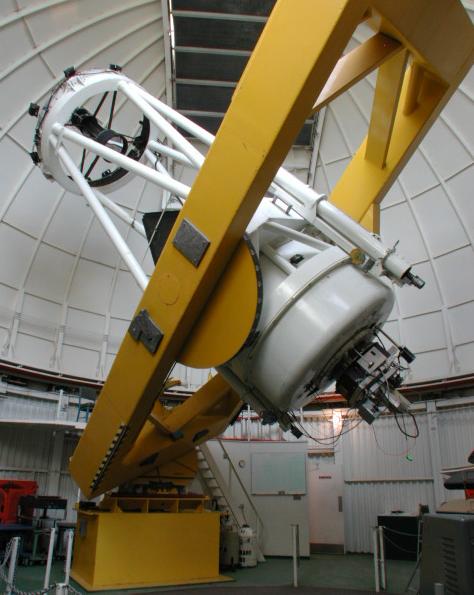The 61" Kuiper telescope. Courtesy Steward Observatory.

The Kuiper is equipped with the Mont4K CCD, which can take data in the Bessel-U, Harris-B, Harris-V, Harris-R, and Arizona-I filters. The filters correspond roughly as follows: U-ultraviolet, B-blue, V-green (visible), R-red, and I-infrared (near-infrared). About half our data has come from the Kuiper.

Much of the rest of our data was gathered on Kitt Peak, at the 90" (2.3m) Bok telescope. The Bok is the largest telescope owned solely by Steward Observatory, and was dedicated in 1969. In 1996 it was named in honor of then Steward Observatory head Professor Bart Bok.

The Bok 90" telescope. Courtesy Wikimedia Commons.

The Bok telescope has instruments that allow for both imaging and spectroscopy. The Bok telescope mainly uses 3 instruments; the 90prime, which does visual-range imaging, the B&C Spectrograph, which does visual spectroscopy, and the Steward 256x256 NIR camera, for infrared observations. Our data comes primarily from the 90prime instrument, although in future observing runs we hope to obtain some spectroscopy data for a relatively recent light-echo candidate supernova. Most of the other half of our data has originated from the Bok telescope.

We have a small amount of data from the Large Binocular Telescope, or LBT, on Mt. Graham. The LBT is one of the world's most advanced optical telescopes, making use of two 27-foot mirrors which together give it the light gathering capability of a single 39-foot mirror and the optical clarity of a 75-foot mirror.

The Large Binocular Telescope. Courtesy Wikimedia Commons.

Although not very much of our data has originated from the LBT due to considerable difficulty in getting observing time on the telescope, the data we do have from there are of unusually high quality.

The last of our data has come from the Holy Grail of telescopes, the Hubble. The data were not, in fact, taken by Dr. Milne but rather in a number of surveys conducted primarily by Nobel Laureate Dr. Adam Riess in searching for cepheids in other galaxies to get a better understanding of the expansion rate of the universe. A few data points are from the HST images, while the other images were primarily used in subtraction.

I have been observing with Dr. Milne at both the Kuiper and Bok telescopes, though our observing targets were not the supernovae that my research focuses on.

In addition to giving an overview of these telescopes, I would also like to briefly introduce the software that Dr. Milne and I have been using for image analysis. It's called IRAF (image reduction and analysis facility), and is a collection of many software components written by the National Optical Astronomy Observatory (NOAO). There are many packages and tasks that IRAF can perform. My roles primarily include fixing bad pixel strips, combining raw data images into stacked, usable data, performing subtraction on images to remove the background field from the supernovae, obtaining useful information about how bright objects are, and plotting the results. Each step involves quite a bit of code and user input, so this analysis is very time consuming. The results, however, tell us all of the information about the light echo I've mentioned previously; brightness, angular size, distance, color, and all the rest. In the past week, I have primarily been focused on stacking the raw images of our 2009 supernova, with some effort being put into subtraction on these same images.

That's all I have for you this week. I hope it wasn't too boring! Thanks for reading, everyone, and tune in next week for another post.